LSTM back propagation: following the flows of variables
First of all, the summary of this article is: please just download my Power Point slides which I made and be patient, following the equations.
I am not supposed to use so many mathematics when I write articles on Data Science Blog. However using little mathematics when I talk about LSTM backprop is like writing German, never caring about “der,” “die,” “das,” or speaking little English in English classes (which most high school English teachers in Japan do) or writing Japanese without using any Chinese characters (which looks like a terrible handwriting by a drug addict). In short, that is ridiculous. And all the precise equations of LSTM backprop, written on a Blog is not a comfortable thing to see. So basically the whole of this article is an advertisement on my PowerPoint slides, sponsored by DATANOMIQ, and I can just give you some tips to get ready for the most tiresome part of understanding LSTM here.
*This article is the fifth article of “A gentle introduction to the tiresome part of understanding RNN.”
*In this article “Densely Connected Layers” is written as “DCL,” and “Convolutional Neural Network” as “CNN.”
1. Chain rules
This article is virtually an article on chain rules of differentiation. Even if you have clear understandings on chain rules, I recommend you to take a look at this section. If you have written down all the equations of back propagation of DCL, you would have seen what chain rules are. Even simple chain rules for backprop of normal DCL can be difficult to some people, but when it comes to backprop of LSTM, it is a pure torture. I think using graphical models would help you understand what chain rules are like. Graphical models are basically used to describe the relations of variables and functions in probabilistic models, so to be exact I am going to use “something like graphical models” in this article. Not that this is a common way to explain chain rules.
First, let’s think about the simplest type of chain rule. Assume that you have a function ![]() , and relations of the functions are displayed as the graphical model at the left side of the figure below. Variables are a type of function, so you should think that every node in graphical models denotes a function. Arrows in purple in the right side of the chart show how information propagate in differentiation.
, and relations of the functions are displayed as the graphical model at the left side of the figure below. Variables are a type of function, so you should think that every node in graphical models denotes a function. Arrows in purple in the right side of the chart show how information propagate in differentiation.

Next, if you a function ![]() , which has two variances
, which has two variances ![]() and
and ![]() . And both of the variances also share two variances
. And both of the variances also share two variances ![]() and
and ![]() . When you take partial differentiation of
. When you take partial differentiation of ![]() with respect to
with respect to ![]() or
or ![]() , the formula is a little tricky. Let’s think about how to calculate
, the formula is a little tricky. Let’s think about how to calculate ![]() . The variance
. The variance ![]() propagates to
propagates to ![]() via
via ![]() and
and ![]() . In this case the partial differentiation has two terms as below.
. In this case the partial differentiation has two terms as below.

In chain rules, you have to think about all the routes where a variance can propagate through. If you generalize chain rules, that is like below, and you need to understand chain rules in this way to understanding any types of back propagation.
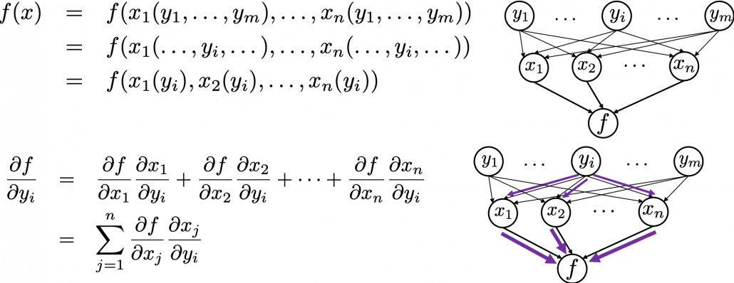
The figure above shows that if you calculate partial differentiation of ![]() with respect to
with respect to ![]() , the partial differentiation has
, the partial differentiation has ![]() terms in total because
terms in total because ![]() propagates to
propagates to ![]() via
via ![]() variances. In order to understand backprop of LSTM, you constantly have to care about the flow of variances, which I showed as arrows in purple above.
variances. In order to understand backprop of LSTM, you constantly have to care about the flow of variances, which I showed as arrows in purple above.
2. Chain rules in LSTM
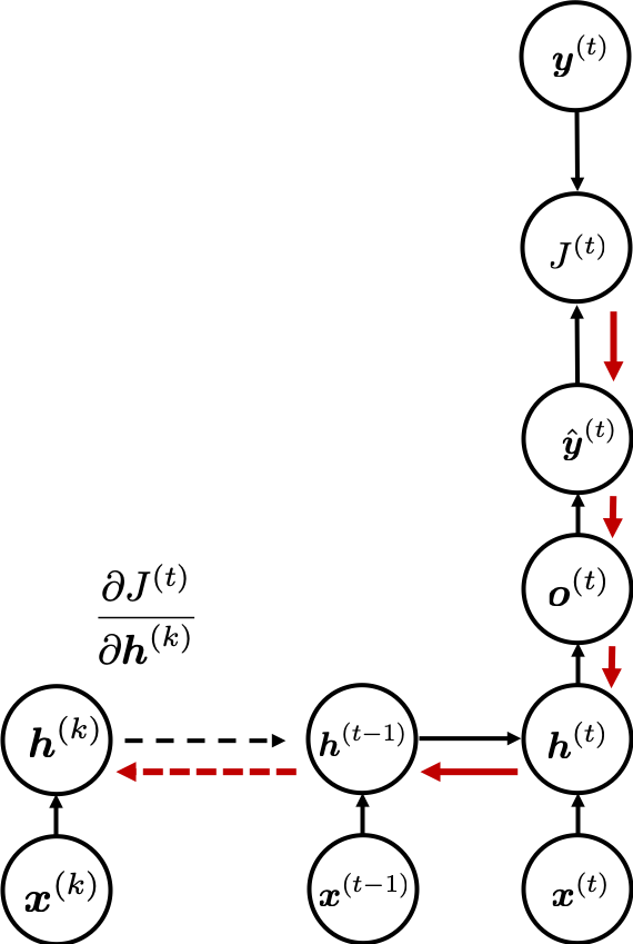
I would like you to remember the figure below, which I used in the second article to show how errors propagate backward during backprop of simple RNNs. After forward propagation, first of all, you need to calculate ![]() , gradients of the error function with respect to parameters, at every time step. But you have to be careful that even though these gradients depend on time steps, the parameters
, gradients of the error function with respect to parameters, at every time step. But you have to be careful that even though these gradients depend on time steps, the parameters ![]() do not depend on time steps.
do not depend on time steps.
*As I mentioned in the second article I personally think ![]() should be rather denoted as
should be rather denoted as ![]() because parameters themselves do not depend on time. The textbook by MIT press also partly use the former notation. And you are likely to encounter this type of notation, so I think it is not bad to get ready for both.
because parameters themselves do not depend on time. The textbook by MIT press also partly use the former notation. And you are likely to encounter this type of notation, so I think it is not bad to get ready for both.
The errors at time step ![]() propagate backward to all the
propagate backward to all the ![]() . Conversely, in order to calculate
. Conversely, in order to calculate ![]() errors flowing from
errors flowing from ![]() . In the chart you need arrows of errors in purple for the gradient in a purple frame, orange arrows for gradients in orange frame, red arrows for gradients in red frame. And you need to sum up
. In the chart you need arrows of errors in purple for the gradient in a purple frame, orange arrows for gradients in orange frame, red arrows for gradients in red frame. And you need to sum up ![]() to calculate
to calculate ![]() , and you need this gradient
, and you need this gradient ![]() to renew parameters, one time.
to renew parameters, one time.
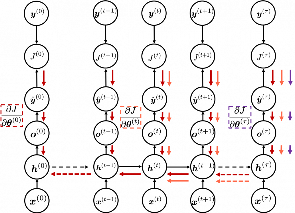
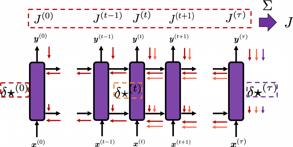
At an RNN block level, the flows of errors and how to renew parameters are the same in LSTM backprop, but the flow of errors inside each block is much more complicated in LSTM backprop. And in this article and my PowerPoint slides, I use a special notation to denote errors: ![]()
* Again, please be careful of what ![]() means. Neurons depend on time steps, but parameters do not depend on time steps. So if
means. Neurons depend on time steps, but parameters do not depend on time steps. So if ![]() are neurons,
are neurons, ![]() , but when
, but when ![]() are parameters,
are parameters, ![]() should be rather denoted like
should be rather denoted like ![]() . In the Space Odyssey paper,
. In the Space Odyssey paper, ![]() are not used as parameters, but in my PowerPoint slides and some other materials,
are not used as parameters, but in my PowerPoint slides and some other materials, ![]() are used also as parameteres.
are used also as parameteres.
As I wrote in the last article, you calculate ![]() as below. Unlike the last article, I also added the terms of peephole connections in the equations below, and I also added the variances
as below. Unlike the last article, I also added the terms of peephole connections in the equations below, and I also added the variances ![]() for convenience.
for convenience.
With Hadamar product operator, the renewed cell and the output are calculated as below.
In this article I would rather give instructions on how to read my PowerPoint slide. Just as general backprop, you need to calculate gradients of error functions with respect to parameters, such as ![]() , where
, where ![]() is either of
is either of ![]() . And just as backprop of simple RNNs, in order to calculate gradients with respect to parameters, you need to calculate errors of neurons, that is gradients of error functions with respect to neurons, such as
. And just as backprop of simple RNNs, in order to calculate gradients with respect to parameters, you need to calculate errors of neurons, that is gradients of error functions with respect to neurons, such as ![]() .
.
*Again and again, keep it in mind that neurons depend on time steps, but parameters do not depend on time steps.
When you calculate gradients with respect to neurons, you can first calculate ![]() , but the equation for this error is the most difficult, so I recommend you to put it aside for now. After calculating
, but the equation for this error is the most difficult, so I recommend you to put it aside for now. After calculating ![]() , you can next calculate
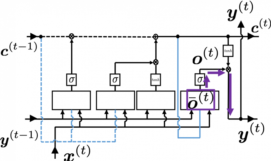
, you can next calculate ![]() . If you see the LSTM block below as a graphical model which I introduced, the information of
. If you see the LSTM block below as a graphical model which I introduced, the information of ![]() flow like the purple arrows. That means,
flow like the purple arrows. That means, ![]() affects
affects ![]() only via
only via ![]() , and this structure is equal to the first graphical model which I have introduced above. And if you calculate
, and this structure is equal to the first graphical model which I have introduced above. And if you calculate ![]() element-wise, you get the equation
element-wise, you get the equation ![]() .
.
*The ![]() is an index of an element of vectors. If you can calculate element-wise gradients, it is easy to understand that as differentiation of vectors and matrices.
is an index of an element of vectors. If you can calculate element-wise gradients, it is easy to understand that as differentiation of vectors and matrices.
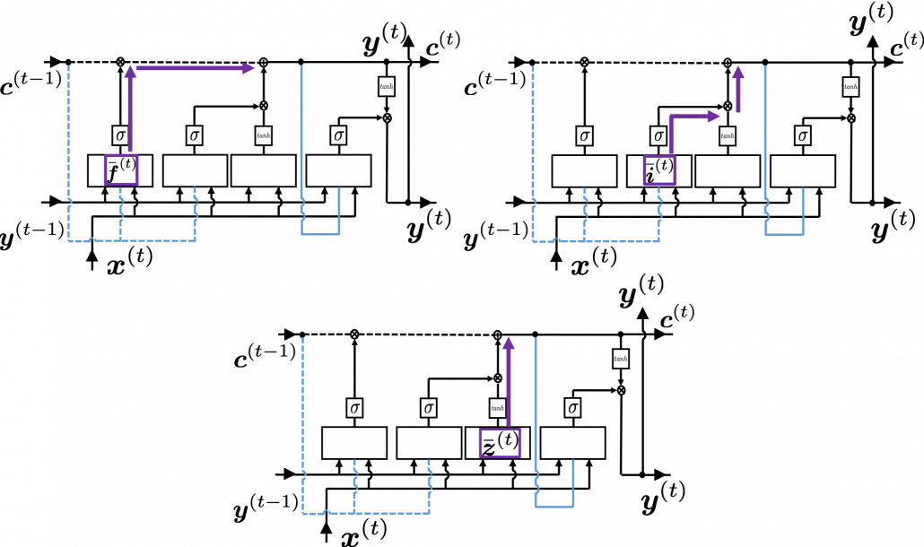
Next you can calculate ![]() , and chain rules are very important in this process. The flow of
, and chain rules are very important in this process. The flow of ![]() to
to ![]() can be roughly divided into two streams: the one flows to
can be roughly divided into two streams: the one flows to ![]() as
as ![]() , and the one flows to
, and the one flows to ![]() as
as ![]() . And the stream from
. And the stream from ![]() to
to ![]() also have two branches: the one via
also have two branches: the one via ![]() and the one which directly converges as
and the one which directly converges as ![]() . Just as well, the stream from
. Just as well, the stream from ![]() to
to ![]() also have three branches: the ones via
also have three branches: the ones via ![]() ,
, ![]() , and the one which directly converges as
, and the one which directly converges as ![]() .
.
If you see see these flows as graphical a graphical model, that would be like the figure below.
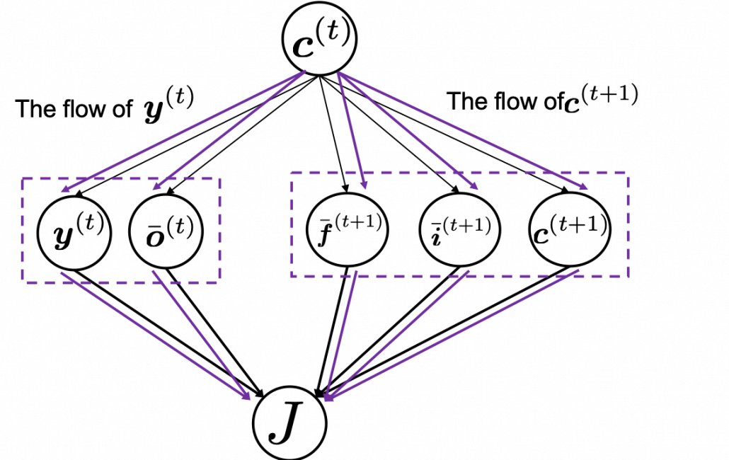
According to this graphical model, you can calculate ![]() element-wise as below.
element-wise as below.
* TO BE VERY HONEST I still do not fully understand why we can apply chain rules like above to calculate ![]() . When you apply the formula of chain rules, which I showed in the first section, to this case, you have to be careful of where to apply partial differential operators
. When you apply the formula of chain rules, which I showed in the first section, to this case, you have to be careful of where to apply partial differential operators ![]() . In the case above, in the part
. In the case above, in the part ![]() the partial differential operator only affects
the partial differential operator only affects ![]() of
of ![]() , and in the part
, and in the part ![]() , the partial differential operator
, the partial differential operator ![]() only affects the part
only affects the part ![]() of the term
of the term ![]() . In the
. In the ![]() part, only
part, only ![]() , in the
, in the ![]() part, only
part, only ![]() , and in the
, and in the ![]() part, only
part, only ![]() . But some other parts, which are not affected by
. But some other parts, which are not affected by ![]() are also functions of
are also functions of ![]() . For example
. For example ![]() of
of ![]() is also a function of
is also a function of ![]() . And I am still not sure about the logic behind where to affect those partial differential operators.
. And I am still not sure about the logic behind where to affect those partial differential operators.
*But at least, these are the only decent equations for LSTM backprop which I could find, and a frequently cited paper on LSTM uses implementation based on these equations. Computer science is more of practical skills, rather than rigid mathematical logic. It If you have any comments or advice on this point, please let me know.
Calculating ![]() ,
, ![]() ,
, ![]() are also relatively straigtforward as calculating
are also relatively straigtforward as calculating ![]() . They all use the first type of chain rule in the first section. Thereby you can get these gradients:
. They all use the first type of chain rule in the first section. Thereby you can get these gradients: ![]() ,
, ![]() , and
, and ![]() .
.
All the gradients which we have calculated use the error ![]() , but when it comes to calculating
, but when it comes to calculating ![]() ….. I can only say “Please be patient. I did my best in my PowerPoint slides to explain that.” It is not a kind of process which I want to explain on Word Press. In conclusion you get an error like this:
….. I can only say “Please be patient. I did my best in my PowerPoint slides to explain that.” It is not a kind of process which I want to explain on Word Press. In conclusion you get an error like this: ![]() , and the flows of
, and the flows of ![]() are as blow.
are as blow.
Combining the gradients we have got so far, we can calculate gradients with respect to parameters. For concrete results, please check the Space Odyssey paper or my PowerPoint slide.
3. How LSTMs tackle exploding/vanishing gradients problems
*If you are allergic to mathematics, you should not read this section or download my PowerPoint slide.
*Part of this section is more or less subjective, so if you really want to know how LSTM mitigate the problems, I highly recommend you to also refer to other materials. But at least I did my best for this article.
LSTMs do not completely solve, vanishing gradient problems. They mitigate vanishing/exploding gradient problems. I am going to roughly explain why they can tackle those problems. I think you find many explanations on that topic, but many of them seems to have some mathematical mistakes (even the slide used in a lecture in Stanford University) and I could not partly agree with some statements. I also could not find any papers or materials which show the whole picture of how LSTMs can tackle those problems. So in this article I am only going to give instructions on the most mainstream way to explain this topic.
First let’s see how gradients actually “vanish” or “explode” in simple RNNs. As I in the second article of this series, simple RNNs propagate forward as the equations below.
And every time step, you get an error function ![]() . Let’s consider the gradient of
. Let’s consider the gradient of ![]() with respect to
with respect to ![]() , that is the error flowing from
, that is the error flowing from ![]() to
to ![]() . This error is the most used to calculate gradients of the parameters.
. This error is the most used to calculate gradients of the parameters.
If you calculate this error more concretely, ![]() , where
, where ![]() .
.
* If you see the figure as a type of graphical model, you should be able to understand the why chain rules can be applied as the equation above.
*According to this paper ![]() , but it seems that many study materials and web sites are mistaken in this point.
, but it seems that many study materials and web sites are mistaken in this point.
Hence  . If you take norms of the members you get an equality
 ![]() . I will not go into detail anymore, but it is known that according to this inequality, multiplication of weight vectors exponentially converge to 0 or to infinite number.
. I will not go into detail anymore, but it is known that according to this inequality, multiplication of weight vectors exponentially converge to 0 or to infinite number.
We have seen that the error ![]() is the main factor causing vanishing/exploding gradient problems. In case of LSTM,
is the main factor causing vanishing/exploding gradient problems. In case of LSTM, ![]() is an equivalent. For simplicity, let’s calculate only
is an equivalent. For simplicity, let’s calculate only ![]() , which is equivalent to
, which is equivalent to ![]() of simple RNN backprop.
of simple RNN backprop.

* Just as I noted above, you have to be careful of which part the partial differential operator ![]() affects in the chain rule above. That is, you need to calculate
affects in the chain rule above. That is, you need to calculate ![]() , and the partial differential operator only affects
, and the partial differential operator only affects ![]() . I think this is not a correct mathematical notation, but please forgive me for doing this for convenience.
. I think this is not a correct mathematical notation, but please forgive me for doing this for convenience.
If you continue calculating the equation above more concretely, you get the equation below.

I cannot mathematically explain why, but it is known that this characteristic of gradients of LSTM backprop mitigate the vanishing/exploding gradient problem. We have seen that if you take a norm of ![]() , that is equal or smaller than repeated multiplication of the norm of the same weight matrix, and that soon leads to vanishing/exploding gradient problem. But according to the equation above, even if you take a norm of repeatedly multiplied
, that is equal or smaller than repeated multiplication of the norm of the same weight matrix, and that soon leads to vanishing/exploding gradient problem. But according to the equation above, even if you take a norm of repeatedly multiplied ![]() , its norm cannot be evaluated with a simple value like repeated multiplication of the norm of the same weight matrix. The outputs of each gate are different from time steps to time steps, and that adjust the value of
, its norm cannot be evaluated with a simple value like repeated multiplication of the norm of the same weight matrix. The outputs of each gate are different from time steps to time steps, and that adjust the value of ![]() .
.
*I personally guess the item ![]() is every effective. The unaffected value of can directly
is every effective. The unaffected value of can directly ![]() adjust the value of
adjust the value of ![]() . And as a matter of fact, it is known that performances of LSTM drop the most when you gite rid of forget gates.
. And as a matter of fact, it is known that performances of LSTM drop the most when you gite rid of forget gates.
When it comes to tackling exploding gradient problems, there is a much easier technique called gradient clipping. This algorithm is very simple: you just have to adjust the size of gradient so that the absolute value of gradient is under a threshold at every time step. Imagine that you decide in which direction to move by calculating gradients, but when the footstep is going to be too big, you just adjust the size of footstep to the threshold size you have set. In a pseudo code, write a gradient clipping part only with two line code as below.

*![]() is a gradient at the time step
is a gradient at the time step ![]() is the maximum size of the “step.”
is the maximum size of the “step.”
The figure below, cited from a deep learning text from MIT press textbook, is a good and straightforward explanation on gradient clipping.It is known that a strongly nonlinear function, such as error functions of RNN, can have very steep or plain areas. If you artificially visualize the idea in 3-dimensional space, as the surface of a loss function ![]() with two variants
with two variants ![]() , that means the loss function
, that means the loss function ![]() has plain areas and very steep cliffs like in the figure.Without gradient clipping, at the left side, you can see that the black dot all of a sudden climb the cliff and could jump to an unexpected area. But with gradient clipping, you avoid such “big jumps” on error functions.
has plain areas and very steep cliffs like in the figure.Without gradient clipping, at the left side, you can see that the black dot all of a sudden climb the cliff and could jump to an unexpected area. But with gradient clipping, you avoid such “big jumps” on error functions.
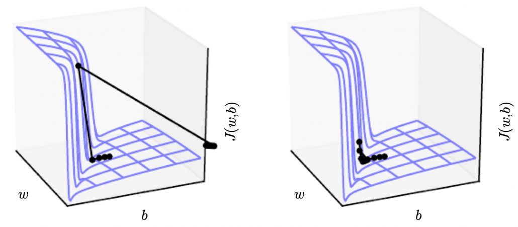
Source: Source: Goodfellow and Yoshua Bengio and Aaron Courville, Deep Learning, (2016), MIT Press, 409p
I am glad that I have finally finished this article series. I am not sure how many of the readers would have read through all of the articles in this series, including my PowerPoint slides. I bet that is not so many. I spent a great deal of my time for making these contents, but sadly even when I was studying LSTM, it was becoming old-fashioned, at least in natural language processing (NLP) field: a very promising algorithm named Transformer has been replacing the position of LSTM. Deep learning is a very fast changing field. I also would like to make illustrative introductions on attention mechanism in NLP, from seq2seq model to Transformer. And I think LSTM would still remain as one of the algorithms in sequence data processing, such as hidden Hidden Markov model, or particle filter.








Leave a Reply
Want to join the discussion?Feel free to contribute!