Seq2seq models and simple attention mechanism: backbones of NLP tasks
This is the second article of my article series “Instructions on Transformer for people outside NLP field, but with examples of NLP.”
1 Machine translation and seq2seq models
I think machine translation is one of the most iconic and commercialized tasks of NLP. With modern machine translation you can translate relatively complicated sentences, if you tolerate some grammatical errors. As I mentioned in the third article of my series on RNN, research on machine translation already started in the early 1950s, and their focus was translation between English and Russian, highly motivated by Cold War. In the initial phase, machine translation was rule-based, like most students do in their foreign language classes. They just implemented a lot of rules for translations. In the next phase, machine translation was statistics-based. They achieved better performance with statistics for constructing sentences. At any rate, both of them highly relied on feature engineering, I mean, you need to consider numerous rules of translation and manually implement them. After those endeavors of machine translation, neural machine translation appeared. The advent of neural machine translation was an earthshaking change of machine translation field. Neural machine translation soon outperformed the conventional techniques, and it is still state of the art. Some of you might felt that machine translation became more or less reliable around that time.

Source: Monty Python’s Life of Brian (1979)
I think you have learnt at least one foreign or classical language in school. I don’t know how good you were at the classes, but I think you had to learn some conjugations of them and I believe that was tiresome to most of students. For example, as a foreign person, I still cannot use “der”, “die”, “das” properly. Some of my friends recommended I do not care them for the time being while I speak, but I usually care grammar very much. But this method of learning language is close to the rule base machine translation, and modern neural machine translation basically does not rely on such rules.
As far as I understand, machine translation is pattern recognition learned from a large corpus. Basically no one implicitly teach computers how grammar works. Machine translation learns very complicated mapping from a source language to a target language, based on a lot of examples of word or sentence pairs. I am not sure, but this might be close to how bilingual kids learn how the two languages are related. You do not need to navigate the translator to learn specific grammatical rules.

Source: Monty Python’s Flying Circus (1969)
Since machine translation does not rely on manually programming grammatical rules, basically you do not need to prepare another specific network architecture for another pair of languages. The same method can be applied to any pairs of languages, as long as you have an enough size of corpus for that. You do not have to think about translation rules between other pairs of languages.

Source: Monty Python’s Flying Circus (1969)
*I do not follow the cutting edge studies on machine translation, so I am not sure, but I guess there are some heuristic methods for machine translation. That is, designing a network depending on the pair of languages could be effective. When it comes grammatical word orders, English and Japanese have totally different structures, I mean English is basically SVO and Japanese is basically SOV. In many cases, the structures of sentences with the same meaning in both of the languages are almost like reflections in a mirror. A lot of languages have similar structures to English, even in Asia, for example Chinese. On the other hand relatively few languages have Japanese-like structures, for example Korean, Turkish. I guess there would be some grammatical-structure-aware machine translation networks.
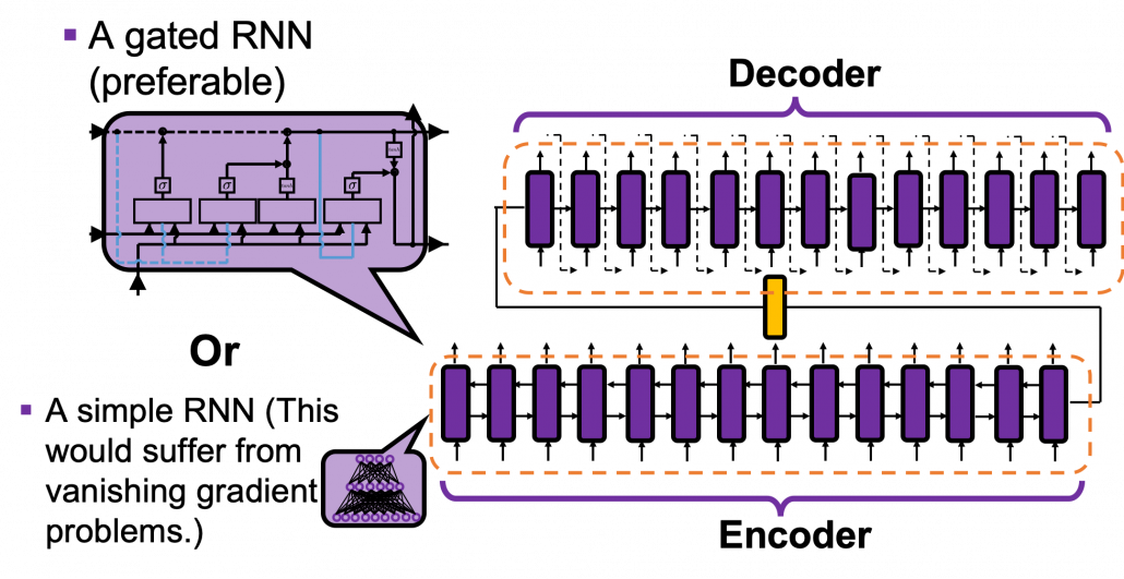
Not only machine translations, but also several other NLP tasks, such as summarization, question answering, use a model named seq2seq model (sequence to sequence model). As well as other deep learning techniques, seq2seq models are composed of an encoder and a decoder. In the case of seq2seq models, you use RNNs in both the encoder and decoder parts. For the RNN cells, you usually use a gated RNN such as LSTM or GRU because simple RNNs would suffer from vanishing gradient problem when inputs or outputs are long, and those in translation tasks are long enough. In the encoder part, you just pass input sentences. To be exact, you input them from the first time step to the last time step, every time giving an output, and passing information to the next cell via recurrent connections.
*I think you would be confused without some understandings on how RNNs propagate forward. You do not need to understand this part that much if you just want to learn Transformer. In order to learn Transformer model, attention mechanism, which I explain in the next section is more important. If you want to know how basic RNNs work, an article of mine should help you.
*In the encoder part of the figure below, the cell also propagate information backward. I assumed an encoder part with bidirectional RNNs, and they “forward propagate” information backwards. But in the codes below, we do not consider such complex situation. Please just keep it in mind that seq2seq model could use bidirectional RNNs.
At the last time step in the encoder part, you pass the hidden state of the RNN to the decoder part, which I show as a yellow cell in the figure below, and the yellow cell/layer is the initial hidden layer of the first RNN cell of the decoder part. Just as normal RNNs, the decoder part start giving out outputs, and passing information via reccurent connections. At every time step you choose a token to give out from the vocabulary you use in the task. That means, each cell of decoder RNNs does a classification task and decides which word to write out at the time step. Also, very importantly, in the decoder part, the output at one time step is the input at the next time step, as I show as dotted lines in the figure below.
*The translation algorithm I explained depends on greedy decoding, which has to decide a token at every time step. However it is easy to imagine that that is not how you translate a word. You usually erase the earlier words or you construct some possibilities in your mind. Actually, for better translations you would need decoding strategies such as beam search, but it is out of the scope of at least this article. Thus we are going to make a very simplified translator based on greedy decoding.
2 Learning by making
*It would take some hours on your computer to train the translator if you do not use a GPU. I recommend you to run it at first and continue reading this article.
Seq2seq models do not have that complicated structures, and for now you just need to understand the points I mentioned above. Rather than just formulating the models, I think it would be better to understand this model by actually writing codes. If you copy and paste the codes in this Github page or the official Tensorflow tutorial, installing necessary libraries, it would start training the seq2seq model for Spanish-English translator. In the Github page, I just added comments to the codes in the official tutorial so that they are more understandable. If you can understand the codes in the tutorial without difficulty, I have to say this article itself is not compatible to your level. Otherwise, I am going to help you understand the tutorial with my original figures. I made this article so that it would help you read the next article. If you have no idea what RNN is, at least the second article of my RNN series should be helpful to some extent.
*If you try to read the the whole article series of mine on RNN, I think you should get prepared. I mean, you should prepare some pieces of paper and a pen. It would be nice if you have some stocks of coffee and snacks. Though I do not think you have to do that to read this article.
2.1 The corpus and datasets
In the codes in the Github page, please ignore the part sandwiched by “######”. Handling language data is not the focus of this article. All you have to know is that the codes below first create datasets from the Spanish-English corpus in http://www.manythings.org/anki/ , and you datasets for training the translator as the tensors below.
Each token is encoded with integers as the codes below, thus after encoding, the Spanish sentence “Todo sobre mi madre.” is [1, 74, 514, 19, 237, 3, 2].
2.2 The encoder
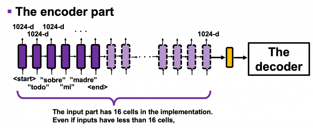
The encoder part is relatively simple. All you have to keep in mind is that you put input sentences, and pass the hidden layer of the last cell to the decoder part. To be more concrete, an RNN cell receives an input word every time step, and gives out an output vector at each time step, passing hidden states to the next cell. You make a chain of RNN cells by the process, like in the figure below. In this case “time steps” means the indexes of the order of the words. If you more or less understand how RNNs work, I think this is nothing difficult. The encoder part passes the hidden state, which is in yellow in the figure below, to the decoder part.
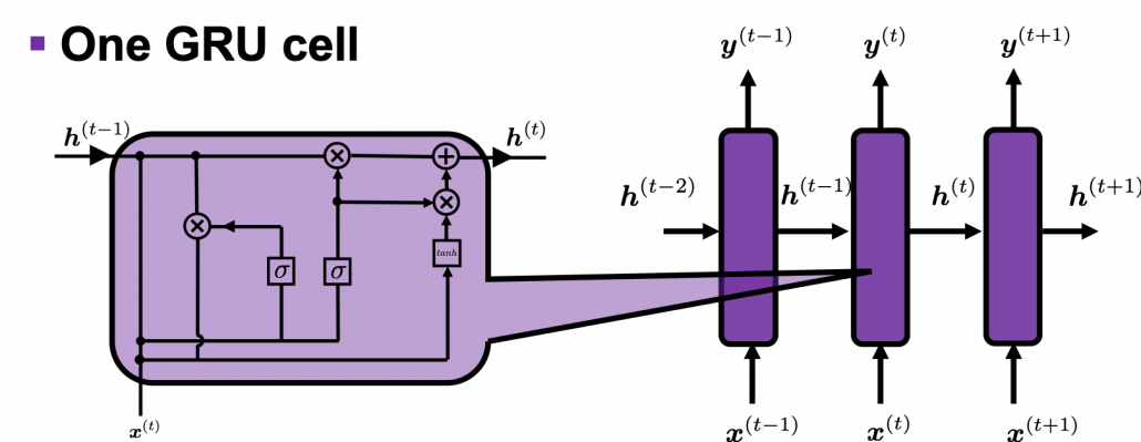
Let’s see how encoders are implemented in the code below. We use a type of RNN named GRU (Gated Recurrent Unit). GRU is simpler than LSTM (Long Short-Term Memory). One GRU cell gets an input every time step, and passes one hidden state via recurrent connections. As well as LSTM, GRU is a gated RNN so that it can mitigate vanishing gradient problems. GRU was invented after LSTM for smaller computation costs. At time step ![]() one GRU cell gets an input
one GRU cell gets an input ![]() and passes its hidden state/vector
and passes its hidden state/vector ![]() to the next cell like the figure below. But in the implementation, you put the whole input sentence as a 16 dimensional vector whose elements are integers, as you saw in the figure in the last subsection 2.1. That means, the ‘Encoder’ class in the implementation below makes a chain of 16 GRU cells every time you put an input sentence in Spanish, even if input sentences have less than 16 tokens.
to the next cell like the figure below. But in the implementation, you put the whole input sentence as a 16 dimensional vector whose elements are integers, as you saw in the figure in the last subsection 2.1. That means, the ‘Encoder’ class in the implementation below makes a chain of 16 GRU cells every time you put an input sentence in Spanish, even if input sentences have less than 16 tokens.
*TO BE VERY HONEST, I am not sure why the encoder part of seq2seq models are implemented this way in the codes below. In the implementation below, the number of total time steps in the encoder part is fixed to 16. If input sentences have less than 16 tokens, it seems the RNN cells get no inputs after the time step of the token “<end>”. As far as I could check, if RNN cells get no inputs, they repeats giving out similar 1024-d vectors. I think in this implementation, RNN cells after the <end> token, which I showed as the dotted RNN cells in the figure above, do not change so much. And the encoder part passes the hidden state of the 16th RNN cell, which is in yellow, to the decoder.
2.3 The decoder
The decoder part is also not that hard to understand. As I briefly explained in the last section, you initialize the first cell of the decoder, using the hidden layer of the last cell the encoder. During decoding, I mean while writing a translation, at the beginning you put the token “<start>” as the first input of the decoder. Given the input “<start>”, the first cell outputs “all” in the example in the figure below, and the output “all” is the input of the next cell. The output of the next cell “about” is also passed to the next cell, and you repeat this till the decoder gives out the token “<end>”.
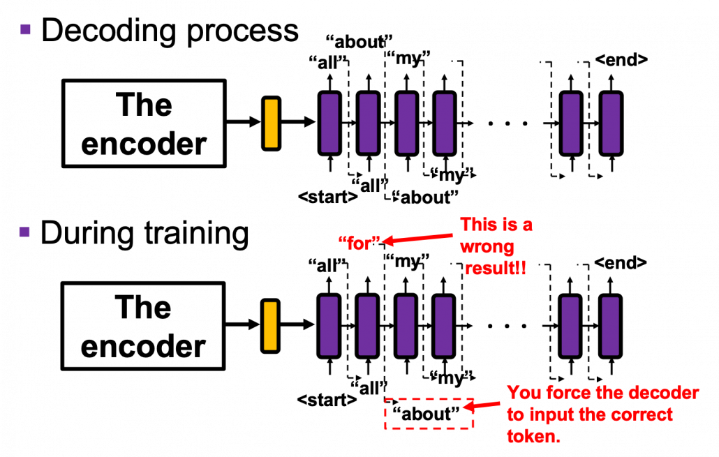
A more important point is how to get losses in the decoder part during training. We use a technique named teacher enforcing during training the decoder part of a seq2seq model. This is also quite simple: you just have to make sure you input a correct answer to RNN cells, regardless of the outputs generated by the cell last time step. You force the decoder to get the correct input every time step, and that is what teacher forcing is all about.
You can see how the decoder part and teacher forcing is implemented in the codes below. You have to keep it in mind that unlike the ‘Encoder’ class, you put a token into a ‘Decoder’ class every time step. To be exact you also need the outputs of the encoder part to calculate attentions in the decoder part. I am going to explain that in the next subsection.
2.4 Attention mechanism
I think you have learned at least one foreign language, and usually you have to translate some sentences. Remember the processes of writing a translation of a sentence in another language. Imagine that you are about to write a new word after writing some. If you are not used to translations in the language, you must have cared about which parts of the original language correspond to the very new word you are going to write. You have to pay “attention” to the original sentence. This is what attention mechanism is all about.
*I would like you to pay “attention” to this section. As you can see from the fact that the original paper on Transformer model is named “Attention Is All You Need,” attention mechanism is a crucial idea of Transformer.
In the decoder part you initialize the hidden layer with the last hidden layer of the encoder, and its first input is “<start>”. The decoder part start decoding, , as I explained in the last subsection. If you use attention mechanism in the seq2seq model, you calculate attentions every times step. Let’s consider an example in the figure below, where the next input in the decoder is “my”, and given the token “my”, the GRU cell calculates a hidden state at the time step. The hidden state is the “query” in this case, and you compare the “query” with the 6 outputs of the encoder, which are “keys”. You get weights/scores, I mean “attentions”, which is the histogram in the figure below.
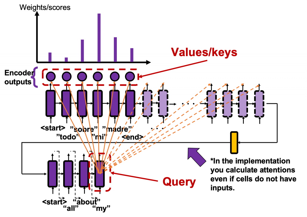 And you reweight the “values” with the weights in the histogram. In this case the “values” are the outputs of the encoder themselves. You used use the reweighted “values” to calculate the hidden state of the decoder at the times step again. And you used the hidden state updated by the attentions to predict the next word.
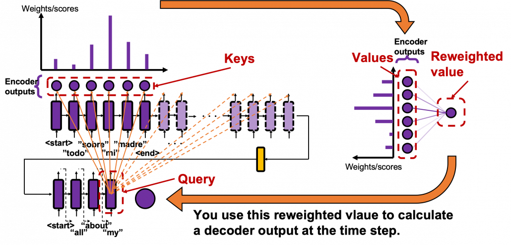
*In the implementation, however, the size of the output of the ‘Encoder’ class is always (16, 2024). You calculate attentions for all those 16 output vectors, but virtually only the first 6 1024-d output vectors important.
Summing up the points I have explained, you compare the “query” with the “keys” and get a scores/weights for the “values.” Each score/weight is in short relevance between the “query” and each “key”. And you reweight the “values” with the scores/weights. In the case of attention mechanism in this article, we can say that “values” and “keys” are the same. You would also see that more clearly in the implementation below.
You especially have to pay attention to the terms “query”, “key”, and “value.” “Keys” and “values” are basically in the same language, and in the case above, they are in Spanish. “Queries” and “keys” can be in either different or the same. In the example above, the “query” is in English, and the “keys” are in Spanish.
You can compare a “query” with “keys” in various ways. The implementation uses the one called Bahdanau’s additive style, and in Transformer, you use more straightforward ways. You do not have to care about how Bahdanau’s additive style calculates those attentions. It is much more important to learn the relations of “queries”, “keys”, and “values” for now.
*A problem is that Bahdanau’s additive style is slightly different from the figure above. It seems in Bahdanau’s additive style, at the time step ![]() in the decoder part, the query is the hidden state at the time step
in the decoder part, the query is the hidden state at the time step ![]() . You would notice that if you closely look at the implementation below.As you can see in the figure above, you can see that you have to calculate the hidden state of the decoder cell two times at the time step
. You would notice that if you closely look at the implementation below.As you can see in the figure above, you can see that you have to calculate the hidden state of the decoder cell two times at the time step ![]() : first in order to generate a “query”, second in order to predict the translated word at the time step. That would not be so computationally efficient, and I guess that is why Bahdanau’s additive style uses the hidden layer at the last time step as a query rather than calculating hidden layers twice.
: first in order to generate a “query”, second in order to predict the translated word at the time step. That would not be so computationally efficient, and I guess that is why Bahdanau’s additive style uses the hidden layer at the last time step as a query rather than calculating hidden layers twice.
2.5 Translating and displaying attentions
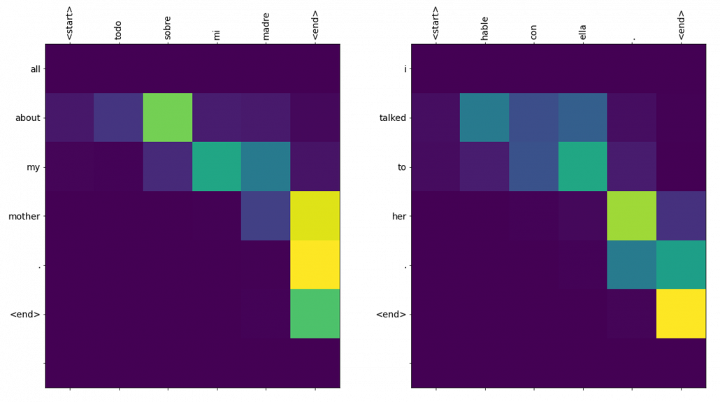
After training the translator for 20 epochs, I could translate Spanish sentences, and the implementation also displays attention scores for between the input and output sentences. For example the translation of the inputs “Todo sobre mi madre.” and “Habre con ella.” were “all about my mother .” and “i talked to her .” respectively, and the results seem fine. One powerful advantage of using attention mechanism is you can display this type of word alignment, I mean correspondences of words in a sentence, easily as in the heat maps below. The yellow parts shows high scores of attentions, and you can see that the distributions of relatively highs scores are more or less diagonal, which implies that English and Spanish have similar word orders.
For other inputs like “Mujeres al borde de un ataque de nervious.” or “Volver.”, the translations are not good.
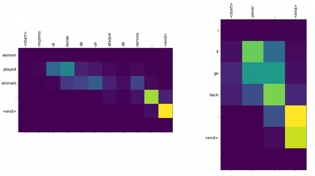
You might have noticed there is one big problem in this implementation: you can use only the words appeared in the corpus. And actually I had to manually add some pairs of sentences with the word “borde” to the corpus to get the translation in the figure.
* I make study materials on machine learning, sponsored by DATANOMIQ. I do my best to make my content as straightforward but as precise as possible. I include all of my reference sources. If you notice any mistakes in my materials, including grammatical errors, please let me know (email: yasuto.tamura@datanomiq.de). And if you have any advice for making my materials more understandable to learners, I would appreciate hearing it.


Leave a Reply
Want to join the discussion?Feel free to contribute!