Language Detecting with sklearn by determining Letter Frequencies

Of course, there are better and more efficient methods to detect the language of a given text than counting its lettes. On the other hand this is a interesting little example to show the impressing ability of todays machine learning algorithms to detect hidden patterns in a given set of data.

For example take the sentence:

“Ceci est une phrase française.”

It’s not to hard to figure out that this sentence is french. But the (lowercase) letters of the same sentence in a random order look like this:

“eeasrsçneticuaicfhenrpaes”

Still sure it’s french? Regarding the fact that this string contains the letter “ç” some people could have remembered long passed french lessons back in school and though might have guessed right. But beside the fact that the french letter “ç” is also present for example in portuguese, turkish, catalan and a few other languages, this is still a easy example just to explain the problem. Just try to guess which language might have generated this:

“ogldviisnntmeyoiiesettpetorotrcitglloeleiengehorntsnraviedeenltseaecithooheinsnstiofwtoienaoaeefiitaeeauobmeeetdmsflteightnttxipecnlgtetgteyhatncdisaceahrfomseehmsindrlttdthoaranthahdgasaebeaturoehtrnnanftxndaeeiposttmnhgttagtsheitistrrcudf”

While this looks simply confusing to the human eye and it seems practically impossible to determine the language it was generated from, this string still contains as set of hidden but well defined patterns from which the language could be predictet with almost complete (ca. 98-99%) certainty.

First of all, we need a set of texts in the languages our model should be able to recognise. Luckily with the package NLTK there comes a big set of example texts which actually are protocolls of the european parliament and therefor are publicly availible in 11 differen languages:

•  Danish
•  Dutch
•  English
•  Finnish
•  French
•  German
•  Greek
•  Italian
•  Portuguese
•  Spanish
•  Swedish

Because the greek version is not written with the latin alphabet, the detection of the language greek would just be too simple, so we stay with the other 10 languages availible. To give you a idea of the used texts, here is a little sample:

“Resumption of the session I declare resumed the session of the European Parliament adjourned on Friday 17 December 1999, and I would like once again to wish you a happy new year in the hope that you enjoyed a pleasant festive period.
Although, as you will have seen, the dreaded ‘millennium bug’ failed to materialise, still the people in a number of countries suffered a series of natural disasters that truly were dreadful.”

Train and Test

The following code imports the nessesary modules and reads the sample texts from a set of text files into a pandas.Dataframe object and prints some statistics about the read texts:

from pathlib import Path
import random
from collections import Counter, defaultdict
import numpy as np
import pandas as pd
from sklearn.neighbors import *
from matplotlib import pyplot as plt
from mpl_toolkits import mplot3d
%matplotlib inline


def read(file):
    '''Returns contents of a file'''
    with open(file, 'r', errors='ignore') as f:
        text = f.read()
    return text

def load_eu_texts():
    '''Read texts snipplets in 10 different languages into pd.Dataframe

    load_eu_texts() -> pd.Dataframe
    
    The text snipplets are taken from the nltk-data corpus.
    '''
    basepath = Path('/home/my_username/nltk_data/corpora/europarl_raw/langs/')
    df = pd.DataFrame(columns=['text', 'lang', 'len'])
    languages = [None]
    for lang in basepath.iterdir():
        languages.append(lang.as_posix())
        t = '\n'.join([read(p) for p in lang.glob('*')])
        d = pd.DataFrame()
        d['text'] = ''
        d['text'] = pd.Series(t.split('\n'))
        d['lang'] = lang.name.title()
        df = df.append(d.copy(), ignore_index=True)
    return df

def clean_eutextdf(df):
    '''Preprocesses the texts by doing a set of cleaning steps
    
    clean_eutextdf(df) -> cleaned_df
    '''
    # Cuts of whitespaces a the beginning and and
    df['text'] = [i.strip() for i in df['text']]
    # Generate a lowercase Version of the text column
    df['ltext'] = [i.lower() for i in df['text']]

    # Determining the length of each text
    df['len'] = [len(i) for i in df['text']]
    # Drops all texts that are not at least 200 chars long
    df = df.loc[df['len'] > 200]
    return df

# Execute the above functions to load the texts
df = clean_eutextdf(load_eu_texts())

# Print a few stats of the read texts
textline = 'Number of text snippplets: ' + str(df.shape[0])
print('\n' + textline + '\n' + ''.join(['_' for i in range(len(textline))]))
c = Counter(df['lang'])
for l in c.most_common():
    print('%-25s' % l[0] + str(l[1]))
df.sample(10)

Number of text snippplets: 56481
________________________________
French                   6466
German                   6401
Italian                  6383
Portuguese               6147
Spanish                  6016
Finnish                  5597
Swedish                  4940
Danish                   4914
Dutch                    4826
English                  4791

lang	len	text	ltext
135233	Finnish	346	Vastustan sitä , toisin kuin tämän parlamentin...	vastustan sitä , toisin kuin tämän parlamentin...
170400	Danish	243	Desuden ødelægger det centraliserede europæisk...	desuden ødelægger det centraliserede europæisk...
85466	Italian	220	In primo luogo , gli accordi di Sharm el-Sheik...	in primo luogo , gli accordi di sharm el-sheik...
15926	French	389	Pour ce qui est concrètement du barrage de Ili...	pour ce qui est concrètement du barrage de ili...
195321	English	204	Discretionary powers for national supervisory ...	discretionary powers for national supervisory ...
160557	Danish	304	Det er de spørgmål , som de lande , der udgør ...	det er de spørgmål , som de lande , der udgør ...
196310	English	355	What remains of the concept of what a company ...	what remains of the concept of what a company ...
110163	Portuguese	327	Actualmente , é do conhecimento dos senhores d...	actualmente , é do conhecimento dos senhores d...
151681	Danish	203	Dette er vigtigt for den tillid , som samfunde...	dette er vigtigt for den tillid , som samfunde...
200540	English	257	Therefore , according to proponents , such as ...	therefore , according to proponents , such as ...

Above you see a sample set of random rows of the created Dataframe. After removing very short text snipplets (less than 200 chars) we are left with 56481 snipplets. The function clean_eutextdf() then creates a lower case representation of the texts in the coloum ‘ltext’ to facilitate counting the chars in the next step.
The following code snipplet now extracs the features – in this case the relative frequency of each letter in every text snipplet – that are used for prediction:

def calc_charratios(df):
    '''Calculating ratio of any (alphabetical) char in any text of df for each lyric
    
    calc_charratios(df) -> list, pd.Dataframe
    '''
    CHARS = ''.join({c for c in ''.join(df['ltext']) if c.isalpha()})
    print('Counting Chars:')
    for c in CHARS:
        print(c, end=' ')
        df[c] = [r.count(c) for r in df['ltext']] / df['len']
    return list(CHARS), df

features, df = calc_charratios(df)

Now that we have calculated the features for every text snipplet in our dataset, we can split our data set in a train and test set:

def split_dataset(df, ratio=0.5):
    '''Split the dataset into a train and a test dataset
    
    split_dataset(featuredf, ratio) -> pd.Dataframe, pd.Dataframe
    '''
    df = df.sample(frac=1).reset_index(drop=True)
    traindf = df[:][:int(df.shape[0] * ratio)]
    testdf = df[:][int(df.shape[0] * ratio):]
    return traindf, testdf

featuredf = pd.DataFrame()
featuredf['lang'] = df['lang']
for feature in features:
    featuredf[feature] = df[feature]
traindf, testdf = split_dataset(featuredf, ratio=0.80)

x = np.array([np.array(row[1:]) for index, row in traindf.iterrows()])
y = np.array([l for l in traindf['lang']])
X = np.array([np.array(row[1:]) for index, row in testdf.iterrows()])
Y = np.array([l for l in testdf['lang']])

After doing that, we can train a k-nearest-neigbours classifier and test it to get the percentage of correctly predicted languages in the test data set. Because we do not know what value for k may be the best choice, we just run the training and testing with different values for k in a for loop:

def train_knn(x, y, k):
    '''Returns the trained k nearest neighbors classifier
    
    train_knn(x, y, k) -> sklearn.neighbors.KNeighborsClassifier
    '''
    clf = KNeighborsClassifier(k)
    clf.fit(x, y)
    return clf

def test_knn(clf, X, Y):
    '''Tests a given classifier with a testset and return result
    
    text_knn(clf, X, Y) -> float
    '''
    predictions = clf.predict(X)
    ratio_correct = len([i for i in range(len(Y)) if Y[i] == predictions[i]]) / len(Y)
    return ratio_correct

print('''k\tPercentage of correctly predicted language
__________________________________________________''')
for i in range(1, 16):
    clf = train_knn(x, y, i)
    ratio_correct = test_knn(clf, X, Y)
    print(str(i) + '\t' + str(round(ratio_correct * 100, 3)) + '%')

k	Percentage of correctly predicted language
__________________________________________________
1	97.548%
2	97.38%
3	98.256%
4	98.132%
5	98.221%
6	98.203%
7	98.327%
8	98.247%
9	98.371%
10	98.345%
11	98.327%
12	98.3%
13	98.256%
14	98.274%
15	98.309%

As you can see in the output the reliability of the language classifier is generally very high: It starts at about 97.5% for k = 1, increases for with increasing values of k until it reaches a maximum level of about 98.5% at k ≈ 10.

Using the Classifier to predict languages of texts

Now that we have trained and tested the classifier we want to use it to predict the language of example texts. To do that we need two more functions, shown in the following piece of code. The first one extracts the nessesary features from the sample text and predict_lang() predicts the language of a the texts:

def extract_features(text, features):
    '''Extracts all alphabetic characters and add their ratios as feature
    
    extract_features(text, features) -> np.array
    '''
    textlen = len(text)
    ratios = []
    text = text.lower()
    for feature in features:
        ratios.append(text.count(feature) / textlen)
    return np.array(ratios)

def predict_lang(text, clf=clf):
    '''Predicts the language of a given text and classifier
    
    predict_lang(text, clf) -> str
    '''
    extracted_features = extract_features(text, features)
    return clf.predict(np.array(np.array([extracted_features])))[0]

text_sample = df.sample(10)['text']

for example_text in text_sample:
    print('%-20s'  % predict_lang(example_text, clf) + '\t' + example_text[:60] + '...')

Italian             	Auspico che i progetti riguardanti i programmi possano contr...
English             	When that time comes , when we have used up all our resource...
Portuguese          	Creio que o Parlamento protesta muitas vezes contra este mét...
Spanish             	Sobre la base de esta posición , me parece que se puede enco...
Dutch               	Ik voel mij daardoor aangemoedigd omdat ik een brede consens...
Spanish             	Señor Presidente , Señorías , antes que nada , quisiera pron...
Italian             	Ricordo altresì , signora Presidente , che durante la preced...
Swedish             	Betänkande ( A5-0107 / 1999 ) av Berend för utskottet för re...
English             	This responsibility cannot only be borne by the Commissioner...
Portuguese          	A nossa leitura comum é que esse partido tem uma posição man...

With this classifier it is now also possible to predict the language of the randomized example snipplet from the introduction (which is acutally created from the first paragraph of this article):

example_text = "ogldviisnntmeyoiiesettpetorotrcitglloeleiengehorntsnraviedeenltseaecithooheinsnstiofwtoienaoaeefiitaeeauobmeeetdmsflteightnttxipecnlgtetgteyhatncdisaceahrfomseehmsindrlttdthoaranthahdgasaebeaturoehtrnnanftxndaeeiposttmnhgttagtsheitistrrcudf"
predict_lang(example_text)
'English'

The KNN classifier of sklearn also offers the possibility to predict the propability with which a given classification is made. While the probability distribution for a specific language is relativly clear for long sample texts it decreases noticeably the shorter the texts are.

def dict_invert(dictionary):
    ''' Inverts keys and values of a dictionary
    
    dict_invert(dictionary) -> collections.defaultdict(list)
    '''
    inverse_dict = defaultdict(list)
    for key, value in dictionary.items():
        inverse_dict[value].append(key)
    return inverse_dict

def get_propabilities(text, features=features):
    '''Prints the probability for every language of a given text
    
    get_propabilities(text, features)
    '''
    results = clf.predict_proba(extract_features(text, features=features).reshape(1, -1))
    for result in zip(clf.classes_, results[0]):
        print('%-20s' % result[0] + '%7s %%' % str(round(float(100 * result[1]), 4)))


example_text = 'ogldviisnntmeyoiiesettpetorotrcitglloeleiengehorntsnraviedeenltseaecithooheinsnstiofwtoienaoaeefiitaeeauobmeeetdmsflteightnttxipecnlgtetgteyhatncdisaceahrfomseehmsindrlttdthoaranthahdgasaebeaturoehtrnnanftxndaeeiposttmnhgttagtsheitistrrcudf'
print(example_text)
get_propabilities(example_text + '\n')
print('\n')
example_text2 = 'Dies ist ein kurzer Beispielsatz.'
print(example_text2)
get_propabilities(example_text2 + '\n')

ogldviisnntmeyoiiesettpetorotrcitglloeleiengehorntsnraviedeenltseaecithooheinsnstiofwtoienaoaeefiitaeeauobmeeetdmsflteightnttxipecnlgtetgteyhatncdisaceahrfomseehmsindrlttdthoaranthahdgasaebeaturoehtrnnanftxndaeeiposttmnhgttagtsheitistrrcudf
Danish                  0.0 %
Dutch                   0.0 %
English               100.0 %
Finnish                 0.0 %
French                  0.0 %
German                  0.0 %
Italian                 0.0 %
Portuguese              0.0 %
Spanish                 0.0 %
Swedish                 0.0 %


Dies ist ein kurzer Beispielsatz.
Danish                  0.0 %
Dutch                   0.0 %
English                 0.0 %
Finnish                 0.0 %
French              18.1818 %
German              72.7273 %
Italian              9.0909 %
Portuguese              0.0 %
Spanish                 0.0 %
Swedish                 0.0 %

Background and Insights

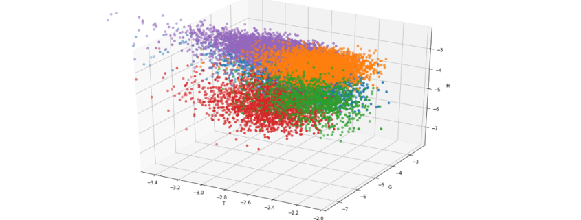
Why does a relative simple model like counting letters acutally work? Every language has a specific pattern of letter frequencies which can be used as a kind of fingerprint: While there are almost no y‘s in the german language this letter is quite common in english. In french the letter k is not very common because it is replaced with q in most cases.

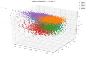
For a better understanding look at the output of the following code snipplet where only three letters already lead to a noticable form of clustering:

projection='3d')
legend = []
X, Y, Z = 'e', 'g', 'h'

def iterlog(ln):
    retvals = []
    for n in ln:
        try:
            retvals.append(np.log(n))
        except:
            retvals.append(None)
    return retvals

for X in ['t']:
    ax = plt.axes(projection='3d')
    ax.xy_viewLim.intervalx = [-3.5, -2]
    legend = []
    for lang in [l for l in df.groupby('lang') if l[0] in {'German', 'English', 'Finnish', 'French', 'Danish'}]:
        sample = lang[1].sample(4000)

        legend.append(lang[0])
        ax.scatter3D(iterlog(sample[X]), iterlog(sample[Y]), iterlog(sample[Z]))

    ax.set_title('log(10) of the Relativ Frequencies of "' + X.upper() + "', '" + Y.upper() + '" and "' + Z.upper() + '"\n\n')
    ax.set_xlabel(X.upper())
    ax.set_ylabel(Y.upper())
    ax.set_zlabel(Z.upper())
    plt.legend(legend)
    plt.show()

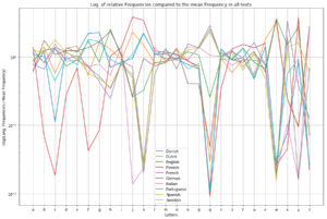
Even though every single letter frequency by itself is not a very reliable indicator, the set of frequencies of all present letters in a text is a quite good evidence because it will more or less represent the letter frequency fingerprint of the given language. Since it is quite hard to imagine or visualize the above plot in more than three dimensions, I used a little trick which shows that every language has its own typical fingerprint of letter frequencies:

legend = []
fig = plt.figure(figsize=(15, 10))
plt.axes(yscale='log')
    
langs = defaultdict(list)

for lang in [l for l in df.groupby('lang') if l[0] in set(df['lang'])]:
    for feature in 'abcdefghijklmnopqrstuvwxyz':
        langs[lang[0]].append(lang[1][feature].mean())

mean_frequencies = {feature:df[feature].mean() for feature in 'abcdefghijklmnopqrstuvwxyz'}
for i in langs.items():
    legend.append(i[0])
    j = np.array(i[1]) / np.array([mean_frequencies[c] for c in 'abcdefghijklmnopqrstuvwxyz'])
    plt.plot([c for c in 'abcdefghijklmnopqrstuvwxyz'], j)
plt.title('Log. of relative Frequencies compared to the mean Frequency in all texts')
plt.xlabel('Letters')
plt.ylabel('(log(Lang. Frequencies / Mean Frequency)')
plt.legend(legend)
plt.grid()
plt.show()

What more?

Beside the fact, that letter frequencies alone, allow us to predict the language of every example text (at least in the 10 languages with latin alphabet we trained for) with almost complete certancy there is even more information hidden in the set of sample texts.

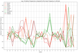
As you might know, most languages in europe belong to either the romanian or the indogermanic language family (which is actually because the romans conquered only half of europe). The border between them could be located in belgium, between france and germany and in swiss. West of this border the romanian languages, which originate from latin, are still spoken, like spanish, portouguese and french. In the middle and northern part of europe the indogermanic languages are very common like german, dutch, swedish ect. If we plot the analysed languages with a different colour sheme this border gets quite clear and allows us to take a look back in history that tells us where our languages originate from:

legend = []
fig = plt.figure(figsize=(15, 10))
plt.axes(yscale='linear')
    
langs = defaultdict(list)
for lang in [l for l in df.groupby('lang') if l[0] in {'German', 'English', 'French', 'Spanish', 'Portuguese', 'Dutch', 'Swedish', 'Danish', 'Italian'}]:
    for feature in 'abcdefghijklmnopqrstuvwxyz':
        langs[lang[0]].append(lang[1][feature].mean())

colordict = {l[0]:l[1] for l in zip([lang for lang in langs], ['brown', 'tomato', 'orangered',
                                                               'green', 'red', 'forestgreen', 'limegreen',
                                                               'darkgreen', 'darkred'])}
mean_frequencies = {feature:df[feature].mean() for feature in 'abcdefghijklmnopqrstuvwxyz'}
for i in langs.items():
    legend.append(i[0])
    j = np.array(i[1]) / np.array([mean_frequencies[c] for c in 'abcdefghijklmnopqrstuvwxyz'])
    plt.plot([c for c in 'abcdefghijklmnopqrstuvwxyz'], j, color=colordict[i[0]])
#     plt.plot([c for c in 'abcdefghijklmnopqrstuvwxyz'], i[1], color=colordict[i[0]])
plt.title('Log. of relative Frequencies compared to the mean Frequency in all texts')
plt.xlabel('Letters')
plt.ylabel('(log(Lang. Frequencies / Mean Frequency)')
plt.legend(legend)
plt.grid()
plt.show()

As you can see the more common letters, especially the vocals like a, e, i, o and u have almost the same frequency in all of this languages. Far more interesting are letters like q, k, c and w: While k is quite common in all of the indogermanic languages it is quite rare in romanic languages because the same sound is written with the letters q or c.
As a result it could be said, that even “boring” sets of data (just give it a try and read all the texts of the protocolls of the EU parliament…) could contain quite interesting patterns which – in this case – allows us to predict quite precisely which language a given text sample is written in, without the need of any translation program or to speak the languages. And as an interesting side effect, where certain things in history happend (or not happend): After two thousand years have passed, modern machine learning techniques could easily uncover this history because even though all these different languages developed, they still have a set of hidden but common patterns that since than stayed the same.

About Author

Christopher Kipp

Christopher Kipp ist Data Scientist bei der DATANOMIQ GmbH. Der studierte Chemiker befasst sich intensiv mit programmatischen und statistischen Lösungen im Bereich Data Science und Data Engineering.

See author's posts